Shape-preserving interpolation method that preserves monotonicity and avoids overshoots.
Math
Statistics
Author
Xuefeng Xu
Published
March 13, 2025
Piecewise Cubic Hermite Interpolating Polynomial (PCHIP) is a cubic spline-based interpolation method designed to preserve monotonicity. See MATLAB or SciPy for the implementation details.
1 PCHIP Example
Given n data points (x_1,y_1),\dots,(x_n,y_n) with x_1<\cdots<x_n, where y is monotonic (either y_i\le y_{i+1} or y_{i+1}\ge y_i). The easiest interpolation method which preserves monotonicity is linear interpolation. However, it is not smooth. Polynomial interpolation is smooth but may introduce overshoots, violating monotonicity.
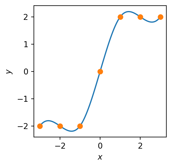
import numpy as npfrom scipy.interpolate import interp1dimport matplotlib.pyplot as pltx = [-3, -2, -1, 0, 1, 2, 3]y = [-6, -5, -1, 0, 1, 5, 6]linear_interp = interp1d(x, y, kind="linear")plot_interp(linear_interp, x, y)cubic_interp = interp1d(x, y, kind="cubic")plot_interp(cubic_interp, x, y)
(a) Linear
(b) Cubic
Figure 1: Linear Interpolation vs. Cubic Interpolation
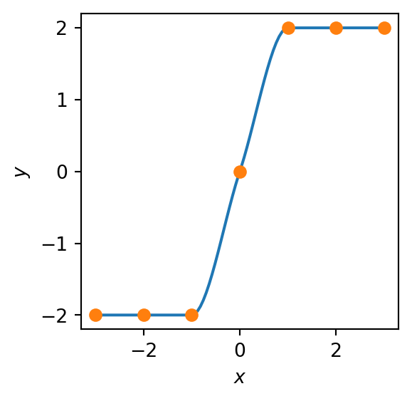
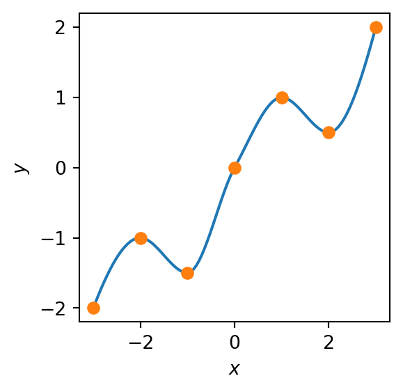
One of the most effective interpolation methods that preserves monotonicity while maintaining smoothness is PCHIP. Some people also refer to it as shape-preserving cubic interpolation. The following figures illustrate PCHIP interpolation, where it also appliable to non-monotonic data points.
Figure 2: PCHIP Interpolation on Monotone and Non-Monotone Data
2 Interpolation Function
How to ensure cubic interpolation preserves monotonicity? Let’s define some notations first. For each interval [x_i,x_{i+1}] (i=1,\dots,n-1), define the step size h_i and slope s_i as:
Thus, computing derivatives d_1,\dots,d_n determines c_0,c_1,c_2,c_3 for each interval.
3 Derivative Formula
The derivative d_i is computed using local information from three neighboring points \{(x_{i-1},y_{i-1}),(x_i,y_i),(x_{i+1},y_{i+1})\}. Replaceing with the slopes s_{i-1} and s_i, and step sizes h_{i-1} and h_i, the formula is (Fritsch and Butland 1984):
A quadratic polynomial \hat{f}(x)=\hat{c}_0+\hat{c}_1x+\hat{c}_2x^2 is fit through the first three points, and \hat{d}_1=\hat{f}'(x_1). Additional rules are then added to preserve monotonicity. Similar procedures apply for d_n.
4 Monotonicity Conditions
To ensure monotonicity, the derivatives d_i must satisfy certain conditions. Define:
To verify Equation 5 and Equation 8 satisfy the monotonicity condition, we analyze them separately. If s_{i-1}s_i>0, then \alpha_i>0; otherwise, \alpha_i=0. Since the ratio r satisfies 1/3<r<2/3, \alpha_i is upper-bounded by 3:
For endpoint \alpha_1, we only need to show the condition of \text{sgn}(\hat{d}_1)=\text{sgn}(s_1)=\text{sgn}(s_2), since other conditions already lie within the region [0,3].
Similarly, \beta_i and endpoint \beta_{n-1} all satisfy the monotonicity condition.
5 Proof of Monotonicity
Proof. To preserve monotonicity, the derivatives d_i and d_{i+1} must align with the direction of the slope of the interval s_i. This is a necessary condition (Fritsch and Carlson 1980):
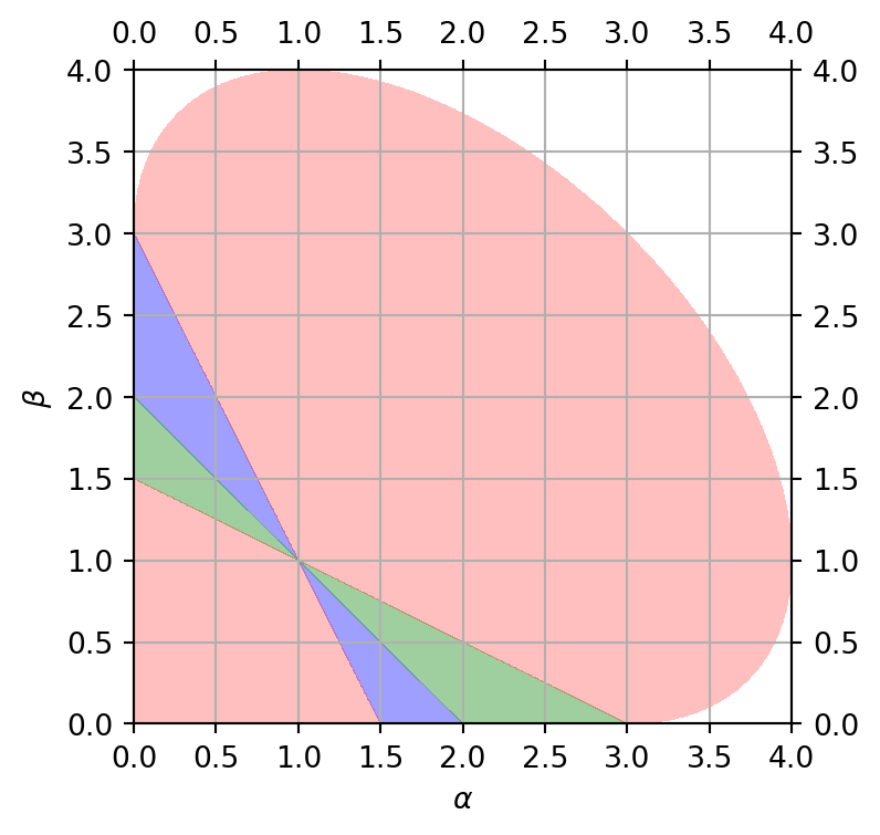
Figure 3 illustrates these conditions: Condition (i) — blue, Condition (ii) — green, Condition (iii) — red.
Code
import numpy as npimport matplotlib.pyplot as pltx_vals = np.linspace(0, 4, 1000)y_vals = np.linspace(0, 4, 1000)x, y = np.meshgrid(x_vals, y_vals)cond1 = (x >0) & (y >0) & ((2* x + y -3) / (x + y -2) <0)cond2 = (x >0) & (y >0) & ((x +2* y -3) / (x + y -2) <0)cond3 = ( (x >0)& (y >0)& ((2* x + y -3) / (x + y -2) >0)& ((x +2* y -3) / (x + y -2) >0)& (x - ((2* x + y -3) **2) / (3* (x + y -2)) >0))fig, ax = plt.subplots(figsize=(3, 3))ax.contourf(x, y, cond1, levels=1, colors=["white", "blue"], alpha=1)ax.contourf(x, y, cond2, levels=1, colors=["white", "green"], alpha=0.5)ax.contourf(x, y, cond3, levels=1, colors=["white", "red"], alpha=0.25)ax.set_xlabel(r"$\alpha$")ax.set_ylabel(r"$\beta$")ax.set_xlim([0, 4])ax.set_ylim([0, 4])ax.xaxis.set_ticks(list(np.arange(0, 4.5, 0.5)))ax.yaxis.set_ticks(list(np.arange(0, 4.5, 0.5)))ax.grid(True)ax.tick_params( bottom=True, top=True, left=True, right=True, labelbottom=True, labeltop=True, labelleft=True, labelright=True,)plt.show()
Figure 3: The monotonicity region
Finally, simplifying yields the final monotonicity condition (Lemma 1).
References
Fritsch, F. N., and J. Butland. 1984. “A Method for Constructing Local Monotone Piecewise Cubic Interpolants.”SIAM Journal on Scientific and Statistical Computing 5 (2): 300–304. https://doi.org/10.1137/0905021.
Fritsch, F. N., and R. E. Carlson. 1980. “Monotone Piecewise Cubic Interpolation.”SIAM Journal on Numerical Analysis 17 (2): 238–46. https://doi.org/10.1137/0717021.