Power Transform

Power transforms are parametric methods that convert data into a Gaussian-like distribution. Two widely used transformations in this category are the Box-Cox (Box and Cox 1964) and Yeo-Johnson (I. Yeo and Johnson 2000) methods, both of which rely on a single parameter \lambda.

1 Two Transformations

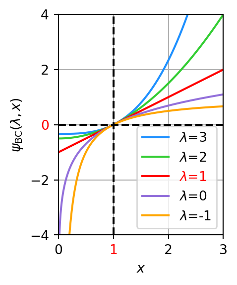
The Box-Cox transformation requires strictly positive data (x > 0) and is defined as:

\psi_{\text{BC}}(\lambda, x) = \begin{cases} \frac{x^\lambda-1}{\lambda} & \text{if } \lambda\neq0,\\ \ln x & \text{if } \lambda=0. \end{cases} \tag{1}

The Yeo-Johnson transformation generalizes Box-Cox to handle non-positive values and is defined as:

\psi_{\text{YJ}}(\lambda, x) = \begin{cases} \frac{(x+1)^\lambda-1}{\lambda} & \text{if } \lambda\neq0,x\ge0,\\ \ln(x+1) & \text{if } \lambda=0,x\ge0,\\ -\frac{(-x+1)^{2-\lambda}-1}{2-\lambda} & \text{if } \lambda\neq2,x<0,\\ -\ln(-x+1) & \text{if } \lambda=2,x<0.\\ \end{cases} \tag{2}

Figure 1 visualizes these transformations across various \lambda values.

import numpy as np
from scipy.special import boxcox
from scipy.stats import yeojohnson
import matplotlib.pyplot as plt

def power_plot(x_min, x_max, power):
    if power == "BC":
        power_func = boxcox
    else:
        power_func = yeojohnson

    eps = 0.01
    x = np.arange(x_min, x_max, eps)

    fig, ax = plt.subplots()
    line_color = ['dodgerblue', 'limegreen', 'red', 'mediumpurple', 'orange']
    for idx, lmb in enumerate([3, 2, 1, 0, -1]):
        y = power_func(x, lmb)
        ax.plot(x, y, label=fr'$\lambda$={lmb}', color=line_color[idx])
    
    ax.set_xlabel(r'$x$')
    if power == "BC":
        ax.set_ylabel(r'$\psi_{\text{BC}}(\lambda, x)$')
    else:
        ax.set_ylabel(r'$\psi_{\text{YJ}}(\lambda, x)$')

    ax.set_xlim(x_min, x_max)
    ax.set_ylim(-4, 4)

    ax.yaxis.set_ticks(list(np.arange(-4, 5, 2)))
    ax.get_yticklabels()[2].set(color="red")
    ax.xaxis.set_ticks(list(np.arange(x_min, x_max + 1)))
    if power == "BC":
        ax.get_xticklabels()[1].set(color="red")
    else:
        ax.get_xticklabels()[2].set(color="red")

    ax.axhline(0, linestyle='--', color='k')
    if power == "BC":
        ax.axvline(1, linestyle='--', color='k')
    else:
        ax.axvline(0, linestyle='--', color='k')

    ax.grid()
    ax.set_aspect(0.5)

    leg = ax.legend(loc='lower right')
    leg.get_texts()[2].set(color="red")

    plt.show()

power_plot(x_min=0, x_max=3, power="BC")
power_plot(x_min=-2, x_max=2, power="YJ")

(a) Box-Cox

(b) Yeo-Johnson

Figure 1: Box-Cox and Yeo-Johnson transformations.

The optimal \lambda is typically estimated by maximizing the log-likelihood. For Box-Cox and Yeo-Johnson, the respective log-likelihood functions are:

\ln\mathcal{L}_{\text{BC}}(\lambda, x)=(\lambda-1) \sum_i^n \ln x_i - \frac{n}{2}\ln\sigma^2_{\psi_{\text{BC}}} \tag{3}

\ln\mathcal{L}_{\text{YJ}}(\lambda, x)=(\lambda-1) \sum_i^n \text{sgn} (x_i) \ln(|x_i|+1) - \frac{n}{2}\ln\sigma^2_{\psi_{\text{YJ}}} \tag{4}

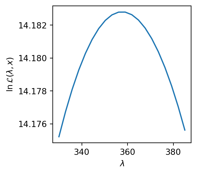
Here, \sigma^2_\psi represents the variance of the transformed data, \text{Var}[\psi(\lambda,x)]. These log-likelihood functions are concave (Kouider and Chen 1995; Marchand et al. 2022), which guarantees a unique maximum. Brent’s method (Brent 2013) is commonly employed for optimization.

from scipy.optimize import brent

def max_llf(x, llf):
    def _neg_llf(lmb, x):
        return -llf(lmb, x)
    return brent(_neg_llf, args=(x,))

2 Numerical Instabilities

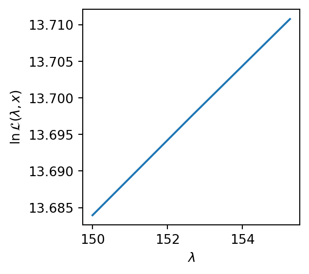
Because both transformations involve exponentiation, they are susceptible to numerical overflow. This problem has been observed by (Marchand et al. 2022) and discussed in Scikit-learn’s GitHub Issue. Below is an example illustrating the problem using a naive implementation of Equation 3:

def boxcox_llf_naive(lmb, x):
    n = len(x)
    logx = np.log(x)
    logvar = np.log(np.var(boxcox(x, lmb)))
    return (lmb - 1) * np.sum(logx) - n/2 * logvar

x = np.array([10, 10, 10, 9.9])
print(max_llf(x, llf=boxcox_llf_naive))

156.48528753755807

/opt/miniconda3/lib/python3.12/site-packages/numpy/_core/_methods.py:194: RuntimeWarning:

overflow encountered in multiply

/opt/miniconda3/lib/python3.12/site-packages/numpy/_core/_methods.py:205: RuntimeWarning:

overflow encountered in reduce

Although this returns a \lambda value, it produces overflow warnings. A useful diagnostic is to visualize the log-likelihood curve:

def plot_llf(x, lb, ub, llf):
    np.set_printoptions(precision=3)
    lmb = np.linspace(lb, ub, 20)
    ll = np.array([llf(l, x) for l in lmb])
    print(f"llf={ll}")

    fig, ax = plt.subplots(figsize=(4, 4))
    ax.plot(lmb, ll)
    ax.set_xlabel(r"$\lambda$")
    ax.set_ylabel(r"$\ln\mathcal{L}(\lambda, x)$")
    plt.show()

plot_llf(x, lb=150, ub=200, llf=boxcox_llf_naive)

llf=[13.684 13.697 13.711   -inf   -inf   -inf   -inf   -inf   -inf   -inf
   -inf   -inf   -inf   -inf   -inf   -inf   -inf   -inf   -inf   -inf]

Unfortunately, due to overflow (np.inf values), the log-likelihood curve cannot be visualized in the specified range, suggesting the returned \lambda is not optimal.

3 Existing Solutions

The MASS package in R (Venables and Ripley 2002) proposes a simple yet effective trick: divide the data by its mean. This rescales the data and avoids numerical instability without affecting the optimization outcome.

x_dm = x / np.mean(x)
print(max_llf(x_dm, llf=boxcox_llf_naive))

357.55141884289054

plot_llf(x_dm, lb=330, ub=385, llf=boxcox_llf_naive)

llf=[23.376 23.377 23.378 23.38  23.381 23.381 23.382 23.383 23.383 23.383
 23.383 23.383 23.383 23.382 23.382 23.381 23.38  23.379 23.377 23.376]

To see why this works, consider the log-variance term for \lambda \ne 0:

\begin{align*} \ln\text{Var}[\psi_{\text{BC}}(\lambda,x)] &=\ln\text{Var}[(x^\lambda-1)/\lambda] \\ &=\ln\text{Var}[x^\lambda/\lambda] \\ &=\ln[\text{Var}(x^\lambda)/\lambda^2] \\ &=\ln\text{Var}(x^\lambda) - 2\ln|\lambda| \\ \end{align*} \tag{5}

If x is scaled by a constant c > 0:

\begin{align*} \ln\text{Var}[\psi_{\text{BC}}(\lambda,x/c)] &=\ln\text{Var}[(x/c)^\lambda] - 2\ln|\lambda| \\ &=\ln[\text{Var}(x^\lambda)/c^{2\lambda}] - 2\ln|\lambda| \\ &=\ln\text{Var}(x^\lambda) - 2\lambda\ln c - 2\ln|\lambda| \\ &=\ln\text{Var}[\psi_{\text{BC}}(\lambda,x)] - 2\lambda\ln c \\ \end{align*} \tag{6}

Plugging into the log−likelihood:

\begin{align*} \ln\mathcal{L}_{\text{BC}}(\lambda, x/c) &=(\lambda-1) \sum_i^n \ln(x_i/c) - \frac{n}{2}\ln\text{Var}[\psi_{\text{BC}}(\lambda,x/c)] \\ &=\ln\mathcal{L}_{\text{BC}}(\lambda, x) - n(\lambda-1)\ln c + n\lambda\ln c \\ &=\ln\mathcal{L}_{\text{BC}}(\lambda, x) + n\ln c \\ \end{align*} \tag{7}

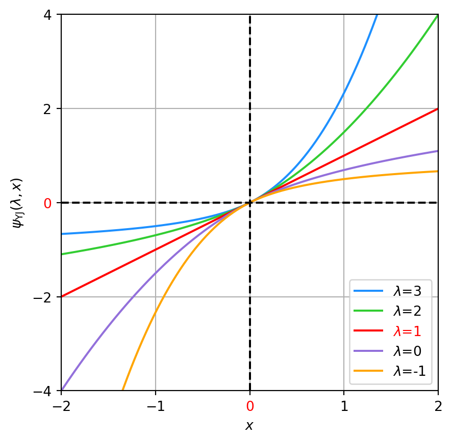
The additive constant n\ln c does not affect the maximizer of \lambda. However, this trick does not apply to Yeo-Johnson, where scaling alters the optimal parameter (see Equation 4).

4 Log-Space Computation

To address numerical instability for both transformations, log-space computation (Haberland 2023) is effective. It uses the Log-Sum-Exp trick to compute statistics in log space:

from scipy.special import logsumexp

def log_mean(logx):
    # compute log of mean of x from log(x)
    return logsumexp(logx) - np.log(len(logx))

def log_var(logx):
    # compute log of variance of x from log(x)
    logmean = log_mean(logx)
    pij = np.full_like(logx, np.pi * 1j, dtype=np.complex128)
    logxmu = logsumexp([logx, logmean + pij], axis=0)
    return np.real(logsumexp(2 * logxmu)) - np.log(len(logx))

This allows direct computation of \ln\sigma^2_\psi from \ln x. Plugging in Equation 5, we can compute the log-likelihood in the log-space.

def boxcox_llf(lmb, x):
    n = len(x)
    logx = np.log(x)
    if lmb == 0:
        logvar = np.log(np.var(logx))
    else:
        logvar = log_var(lmb * logx) - 2 * np.log(abs(lmb))
    return (lmb - 1) * np.sum(logx) - n/2 * logvar

This version avoids overflow and reliably returns the optimal \lambda.

print(max_llf(x, llf=boxcox_llf))

357.55141245531865

plot_llf(x, lb=330, ub=385, llf=boxcox_llf)

llf=[14.175 14.177 14.178 14.179 14.18  14.181 14.182 14.182 14.183 14.183
 14.183 14.183 14.182 14.182 14.181 14.18  14.179 14.178 14.177 14.176]

The same principle extends to Yeo-Johnson, even for mixed-sign inputs.

def log_var_yeojohnson(x, lmb):
    if np.all(x >= 0):
        if abs(lmb) < np.spacing(1.0):
            return np.log(np.var(np.log1p(x)))
        return log_var(lmb * np.log1p(x)) - 2 * np.log(abs(lmb))

    elif np.all(x < 0):
        if abs(lmb - 2) < np.spacing(1.0):
            return np.log(np.var(np.log1p(-x)))
        return log_var((2 - lmb) * np.log1p(-x)) - 2 * np.log(abs(2 - lmb))

    else:  # mixed positive and negtive data
        logyj = np.zeros_like(x, dtype=np.complex128)
        pos = x >= 0

        # when x >= 0
        if abs(lmb) < np.spacing(1.0):
            logyj[pos] = np.log(np.log1p(x[pos]) + 0j)
        else:  # lmbda != 0
            logm1_pos = np.full_like(x[pos], np.pi * 1j, dtype=np.complex128)
            logyj[pos] = logsumexp(
                [lmb * np.log1p(x[pos]), logm1_pos], axis=0
            ) - np.log(lmb + 0j)

        # when x < 0
        if abs(lmb - 2) < np.spacing(1.0):
            logyj[~pos] = np.log(-np.log1p(-x[~pos]) + 0j)
        else:  # lmbda != 2
            logm1_neg = np.full_like(x[~pos], np.pi * 1j, dtype=np.complex128)
            logyj[~pos] = logsumexp(
                [(2 - lmb) * np.log1p(-x[~pos]), logm1_neg], axis=0
            ) - np.log(lmb - 2 + 0j)

        return log_var(logyj)

def yeojohnson_llf(lmb, x):
    n = len(x)
    llf = (lmb - 1) * np.sum(np.sign(x) * np.log1p(np.abs(x)))
    llf += -n / 2 * log_var_yeojohnson(x, lmb)
    return llf

5 Constrained Optimization

Even with log-space computation, applying the transformation using a large absolute value of \lambda can result in overflow:

lmax = max_llf(x, llf=boxcox_llf)
print(boxcox(x, lmax))

[inf inf inf inf]

To prevent this, we constrain \lambda so that the transformed values stay within a safe range.

Lemma 1 The transformation \psi(\lambda,x) is monotonically increasing in both \lambda and x (see I.-K. Yeo 1997 for Yeo-Johnson proof).

This allows us to bound \lambda based on \min(x) and \max(x). For Box-Cox, we use x=1 as a threshold since \psi_\text{BC}(\lambda,1)=0:

\begin{align*} \max_\lambda \quad & \ln\mathcal{L}_{\text{BC}}(\lambda, x) \\ \textrm{s.t.} \quad & \text{if } x_{\max}>1, \lambda\le\psi^{-1}_{\text{BC}}(x_{\max},y_{\max}) \\ & \text{if } x_{\min}<1, \lambda\ge\psi^{-1}_{\text{BC}}(x_{\min},-y_{\max}) \\ \end{align*} \tag{8}

The inverse Box−Cox function is given by:

\psi^{-1}_{\text{BC}}(x,y)=-1/y-W(-x^{-1/y}\ln x/y)/\ln x \tag{9}

from scipy.special import lambertw

def boxcox_inv_lmbda(x, y):
    num = lambertw(-(x ** (-1 / y)) * np.log(x) / y, k=-1)
    return -1 / y - np.real(num / np.log(x))

def boxcox_constranined_lmax(lmax, x, ymax):
    # x > 1, boxcox(x) > 0; x < 1, boxcox(x) < 0
    xmin, xmax = min(x), max(x)
    if xmin >= 1:
        x_treme = xmax
    elif xmax <= 1:
        x_treme = xmin
    else:  # xmin < 1 < xmax
        indicator = boxcox(xmax, lmax) > abs(boxcox(xmin, lmax))
        x_treme = xmax if indicator else xmin
    
    if abs(boxcox(x_treme, lmax)) > ymax:
        lmax = boxcox_inv_lmbda(x_treme, ymax * np.sign(x_treme - 1))
    return lmax

This method can be verified by testing different values for y_{\max}:

def verify_boxcox_constranined_lmax(x):
    np.set_printoptions(precision=3)
    lmax = max_llf(x, llf=boxcox_llf)
    for ymax in [1e300, 1e100, 1e30, 1e10]:
        l = boxcox_constranined_lmax(lmax, x, ymax)
        print(boxcox(x, l))

# Positive overflow
x = np.array([10, 10, 10, 9.9])
verify_boxcox_constranined_lmax(x)

[1.000e+300 1.000e+300 1.000e+300 4.783e+298]
[1.000e+100 1.000e+100 1.000e+100 3.587e+099]
[1.000e+30 1.000e+30 1.000e+30 7.286e+29]
[1.00e+10 1.00e+10 1.00e+10 8.95e+09]

# Negative overflow
x = np.array([0.1, 0.1, 0.1, 0.101])
verify_boxcox_constranined_lmax(x)

[-1.00e+300 -1.00e+300 -1.00e+300 -4.93e+298]
[-1.000e+100 -1.000e+100 -1.000e+100 -3.624e+099]
[-1.000e+30 -1.000e+30 -1.000e+30 -7.309e+29]
[-1.000e+10 -1.000e+10 -1.000e+10 -8.959e+09]

The constrained optimization approach can also be extended to Yeo-Johnson, ensures overflow-free transformations even for extreme values.

def yeojohnson_inv_lmbda(x, y):
    if x >= 0:
        num = lambertw(-((x + 1) ** (-1 / y) * np.log1p(x)) / y, k=-1)
        return -1 / y + np.real(-num / np.log1p(x))
    else:
        num = lambertw(((1 - x) ** (1 / y) * np.log1p(-x)) / y, k=-1)
        return -1 / y + 2 + np.real(num / np.log1p(-x))

def yeojohnson_constranined_lmax(lmax, x, ymax):
    # x > 0, yeojohnson(x) > 0; x < 0, yeojohnson(x) < 0
    xmin, xmax = min(x), max(x)
    if xmin >= 0:
        x_treme = xmax
    elif xmax <= 0:
        x_treme = xmin
    else:  # xmin < 0 < xmax
        with np.errstate(over="ignore"):
            indicator = yeojohnson(xmax, lmax) > abs(yeojohnson(xmin, lmax))
        x_treme = xmax if indicator else xmin

    with np.errstate(over="ignore"):
        if abs(yeojohnson(x_treme, lmax)) > ymax:
            lmax = yeojohnson_inv_lmbda(x_treme, ymax * np.sign(x_treme))
    return lmax

References

Box, G. E. P., and D. R. Cox. 1964. “An Analysis of Transformations.” Journal of the Royal Statistical Society: Series B (Methodological) 26 (2): 211–43. https://doi.org/10.1111/j.2517-6161.1964.tb00553.x.

Brent, Richard P. 2013. Algorithms for Minimization Without Derivatives. Dover Books on Mathematics. Dover Publications, Incorporated.

Haberland, Matt. 2023. https://github.com/scipy/scipy/pull/18852#issuecomment-1657858886.

Kouider, Elies, and Hanfeng Chen. 1995. “Concavity of Box-Cox Log-Likelihood Function.” Statistics & Probability Letters 25 (2): 171–75. https://doi.org/10.1016/0167-7152(94)00219-X.

Marchand, Tanguy, Boris Muzellec, Constance Béguier, Jean Ogier du Terrail, and Mathieu Andreux. 2022. “SecureFedYJ: A Safe Feature Gaussianization Protocol for Federated Learning.” In Advances in Neural Information Processing Systems, 35:36585–98. Curran Associates, Inc. https://doi.org/10.48550/arXiv.2210.01639.

Venables, W. N., and B. D. Ripley. 2002. Modern Applied Statistics with s. Fourth. New York: Springer. https://doi.org/10.32614/CRAN.package.MASS.

Yeo, In-Kwon. 1997. “A New Family of Power Transformations to Reduce Skewness or Approximate Normality.” PhD thesis, The University of Wisconsin-Madison. https://www.proquest.com/openview/b7835693052aecd65e635d39a6bd099a/.

Yeo, In‐Kwon, and Richard A. Johnson. 2000. “A New Family of Power Transformations to Improve Normality or Symmetry.” Biometrika 87 (4): 954–59. https://doi.org/10.1093/biomet/87.4.954.