ROC and PR Curves

Receiver Operating Characteristic (ROC) and Precision–Recall (PR) curves are essential for evaluating classification models. They visualize trade-offs between True Positive Rate (TPR) and False Positive Rate (FPR) (ROC) or Precision and Recall (PR), offering deeper insights than single scalar metrics.

1 ROC Curve

For binary classification, with Positive (P) and Negative (N) classes, predictions are based on model scores thresholded to produce labels. Performance is summarized using a confusion matrix (Table 1), counting True Positives (TP), False Positives (FP), True Negatives (TN), and False Negatives (FN).

Table 1: The Confusion Matrix

Total=P+N	Predicted Pos (PP)	Predicted Neg (PN)
Actual Pos (P)	TP	FN	P=TP+FN
Actual Neg (N)	FP	TN	N=FP+TN
	PP=TP+FP	PN=FN+TN

The ROC curve plots TPR vs. FPR, where:

\text{TPR}=\text{TP}/\text{P},\quad \text{FPR}=\text{FP}/\text{N} \tag{1}

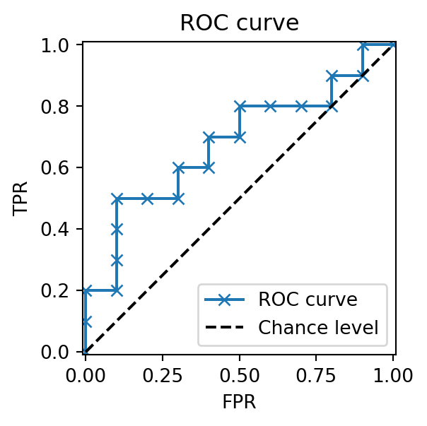
A simple algorithm constructs the ROC curve: 1) Sort predictions in descending score order. 2) Sweep thresholds across scores, updating TP and FP counts (Fawcett 2006).

import numpy as np

def count_fp_tp(y_true, y_score):
    fp, tp = 0, 0
    fps, tps, thresholds = [], [], []
    score = np.inf

    for i in np.flip(np.argsort(y_score)):
1        if y_score[i] != score:
            fps.append(fp)
            tps.append(tp)
            thresholds.append(score)
            score = y_score[i]

        if y_true[i] == 1:
            tp += 1
        else:
            fp += 1

    fps.append(fp)
    tps.append(tp)
    thresholds.append(score)
    return np.asarray(fps), np.asarray(tps), np.asarray(thresholds)

def roc_curve(y_true, y_score):
    fps, tps, thresholds = count_fp_tp(y_true, y_score)
    fpr = fps / sum(y_true == 0)
    tpr = tps / sum(y_true == 1)
    return fpr, tpr, thresholds

1

To handle score repetitions, record (FP, TP) counts only when the score changes.

The ROC curve is always monotonically non-decreasing, starting at (0, 0) for the highest threshold and ending at (1, 1) for the lowest threshold. Points are connected using linear interpolation. A random classifier lies along y=x, while curves closer to the top-left indicate better performance.

import matplotlib.pyplot as plt

def plot_curve(x, y, curve: str, pos_frac=None, drawstyle="default", ax=None):
    if ax is None:
        _, ax = plt.subplots()

    name = f"{curve} curve"
    ax.plot(x, y, "x-", c="C0", label=name, drawstyle=drawstyle)
    ax.set_title(name)

    ax.set_aspect("equal")
    ax.set_xlim(-0.01, 1.01)
    ax.set_ylim(-0.01, 1.01)
    
    chance = {
        "label": "Chance level",
        "color": "k",
        "linestyle": "--",
    }
    if curve == "ROC":
        ax.plot([0, 1], [0, 1], **chance)
        ax.set_xlabel("FPR")
        ax.set_ylabel("TPR")
        ax.legend(loc="lower right")
    elif curve == "PR":  # curve == "PR":
        if pos_frac is not None:
            ax.plot([0, 1], [pos_frac, pos_frac], **chance)
        ax.set_xlabel("Recall")
        ax.set_ylabel("Precision")
        ax.legend(loc="lower left")
    elif curve == "PRG":
        ax.set_xlabel("Recall Gain")
        ax.set_ylabel("Precision Gain")
        ax.legend(loc="lower left")
    else:
        raise ValueError(f"Unknown curve type: {curve}")

y_true = np.array([1, 1, 0, 1, 1, 1, 0, 0, 1, 0, 1, 0, 1, 0, 0, 0, 1, 0, 1, 0])
y_score = np.array([
    .9, .8, .7, .6, .55, .54, .53, .52, .51, .505,
    .4, .39, .38, .37, .36, .35, .34, .33, .3, .1
])

fpr, tpr, _ = roc_curve(y_true, y_score)
plot_curve(fpr, tpr, "ROC")

2 ROC Convex Hull

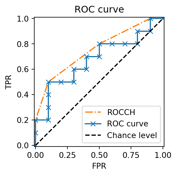
The ROC Convex Hull (ROCCH) highlights potentially optimal performance of a classifier (or a set of classifiers) by connecting upper boundary points (Provost and Fawcett 2001). It can be computed via algorithms like the Monotone chain algorithm.

def convex_hull(points):
    points = sorted(set(points))

    def cross(o, a, b):
        return (a[0] - o[0]) * (b[1] - o[1]) - (a[1] - o[1]) * (b[0] - o[0])

    # Build upper hull
    upper = []
    for p in reversed(points):
        while len(upper) >= 2 and cross(upper[-2], upper[-1], p) <= 0:
            upper.pop()
        upper.append(p)
    
    return upper

rocch = convex_hull(zip(fpr, tpr))

rocch = np.array(rocch)
fpr_ch, tpr_ch = rocch[:, 0], rocch[:, 1]

fig, ax = plt.subplots()
ax.plot(fpr_ch, tpr_ch, 'C1-.', label="ROCCH")
plot_curve(fpr, tpr, "ROC", ax=ax)

3 PR Curve

PR curves plot Precision vs. Recall. Recall equals TPR, while Precision is:

\text{Prec}=\frac{\text{TP}}{\text{TP}+\text{FP}} \tag{2}

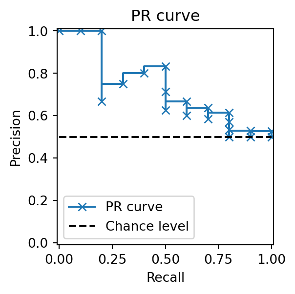
PR curves start at (0, 1) and end at (1, \frac{\text{P}}{\text{P}+\text{N}}), where the endpoint reflects the proportion of positive samples. Because Precision depends on both TP and FP, the PR curve is non-monotonic and can decrease as Recall increases. Moreover, it is highly influenced by class imbalance (Williams 2021). For a random classifier, the PR curve is a horizontal line at y = \frac{\text{P}}{\text{P}+\text{N}}, whereas curves closer to the top-right indicate stronger performance.

def pr_curve(y_true, y_score):
    fps, tps, thresholds = count_fp_tp(y_true, y_score)

    pps = fps + tps
    precision = np.ones_like(tps, dtype=np.float64)
    np.divide(tps, pps, out=precision, where=(pps != 0))

    recall = tps / sum(y_true == 1)
    return np.flip(precision), np.flip(recall), np.flip(thresholds)

Although ROC and PR curves are mathematically related, linear interpolation is incorrect for PR curves, as it yields overly optimistic estimates of performance (Davis and Goadrich 2006). Precision does not necessarily vary linearly with Recall, so naive interpolation misrepresents true model behavior.

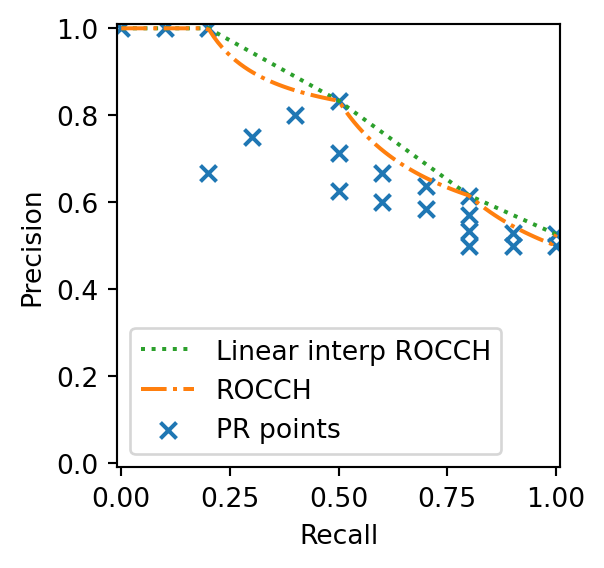
To illustrate this, we convert the ROC Convex Hull (ROCCH) into PR space, treating it as the potential optimal PR curve. Using Equation 3, we express Precision in terms of TPR and FPR:

\text{Prec}=\frac{\text{P}\cdot\text{TPR}}{\text{P}\cdot\text{TPR}+\text{N}\cdot\text{FPR}} =\frac{1}{1+\frac{\text{N}}{\text{P}}\cdot\frac{\text{FPR}}{\text{TPR}}} \tag{3}

from scipy.interpolate import interp1d

def pr_from_roc(fpr, tpr, neg_to_pos):
    fpr_tpr_func = interp1d(tpr, fpr, bounds_error=False, fill_value=(0, 1))

    def prec_func(tpr):
        fpr = fpr_tpr_func(tpr)
        fpr_to_tpr = np.zeros_like(tpr, dtype=np.float64)
        np.divide(fpr, tpr, out=fpr_to_tpr, where=(tpr != 0))
        prec = 1 / (1 + neg_to_pos * fpr_to_tpr)
        return prec

    return prec_func

neg_to_pos = sum(y_true == 0) / sum(y_true == 1)
prec_ch_func = pr_from_roc(fpr_ch, tpr_ch, neg_to_pos)

fig, ax = plt.subplots()
ax.plot(tpr_ch, prec_ch_func(tpr_ch), 'C2:', label="Linear interp ROCCH")

x = np.linspace(0, 1, 100)
ax.plot(x, prec_ch_func(x), 'C1-.', label="ROCCH")

precision, recall, _ = pr_curve(y_true, y_score)
ax.scatter(recall, precision, c="C0", marker="x", label="PR points")

ax.set_aspect("equal")
ax.set_xlim(-0.01, 1.01)
ax.set_ylim(-0.01, 1.01)
ax.set_xlabel("Recall")
ax.set_ylabel("Precision")
ax.legend(loc="lower left")

The converted ROCCH dominates the PR space but is clearly non-linear, lying beneath its own linear interpolation (dotted line). This confirms that PR curves cannot be linearly interpolated. Scikit-learn’s PrecisionRecallDisplay instead uses step-wise interpolation, consistent with average_precision_score. This ensures that the area under the PR curve equals the average precision.

pos_frac = sum(y_true == 1) / len(y_true)
plot_curve(recall, precision, "PR", pos_frac, drawstyle="steps-post")

4 PRG Curve

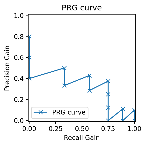
ROC curves benefit from linear interpolation and universal baselines, whereas PR curves lack these properties. To address this, Flach and Kull (2015) proposed the Precision–Recall-Gain (PRG) curve, which transforms Precision and Recall into Gains and plots these Precision Gain and Recall Gain within the unit square:

\text{PrecG}=\frac{\text{Prec}-\pi}{(1-\pi)\text{Prec}},\quad \text{RecG}=\frac{\text{Rec}-\pi}{(1-\pi)\text{Rec}} \tag{4}

where \pi=\frac{\text{P}}{\text{P}+\text{N}} is the positive class fraction. Notably, Gains can be negative, and such points are typically omitted from the PRG curve.

def prg_curve(y_true, y_score):
    prec, rec, thresholds = pr_curve(y_true, y_score)
    pos_frac = sum(y_true == 0) / len(y_true)

    # Remove negative gains
    mask = (rec >= pos_frac) & (prec >= pos_frac)
    prec = prec[mask]
    rec = rec[mask]

    prec_gain = (prec - pos_frac) / (1 - pos_frac) / prec
    rec_gain = (rec - pos_frac) / (1 - pos_frac) / rec
    return prec_gain, rec_gain, thresholds

prec_gain, rec_gain, _ = prg_curve(y_true, y_score)
plot_curve(rec_gain, prec_gain, "PRG")

References

Davis, Jesse, and Mark Goadrich. 2006. “The Relationship Between Precision-Recall and ROC Curves.” In Proceedings of the 23rd International Conference on Machine Learning, 233–40. ICML ’06. New York, NY, USA: Association for Computing Machinery. https://doi.org/10.1145/1143844.1143874.

Fawcett, Tom. 2006. “An Introduction to ROC Analysis.” Pattern Recognition Letters 27 (8): 861–74. https://doi.org/10.1016/j.patrec.2005.10.010.

Flach, Peter, and Meelis Kull. 2015. “Precision-Recall-Gain Curves: PR Analysis Done Right.” In Advances in Neural Information Processing Systems. Vol. 28. Curran Associates, Inc. https://papers.nips.cc/paper/5867-precision-recall-gain-curves-pr-analysis-done-right.

Provost, Foster J., and Tom Fawcett. 2001. “Robust Classification for Imprecise Environments.” Machine Learning 42 (3): 203–31. https://doi.org/10.1023/A:1007601015854.

Williams, Christopher K. I. 2021. “The Effect of Class Imbalance on Precision-Recall Curves.” Neural Computation 33 (4): 853–57. https://doi.org/10.1162/neco_a_01362.