How to Compute Variance?

Given a dataset \{x_1, \ldots, x_n\}, variance measures how much data points deviate from their mean. While the mathematical definition is straightforward, the way we implement variance can have a big impact on numerical stability.

1 Textbook Formulas

The most common definition computes the mean first, then the average squared deviation from it:

\mu = \frac{1}{n} \sum_{i=1}^n x_i,\ \sigma^2 = \frac{1}{n} \sum_{i=1}^n (x_i - \mu)^2. \tag{1}

def var_twopass_textbook(x):
    n, s = 0, 0
    for xi in x:
        n += 1
        s += xi

    mu = s / n
    sd = 0
    for xi in x:
        sd += (xi - mu) ** 2
    return sd / n

This requires two passes over the data. For streaming or memory-constrained scenarios, a one-pass formula is often considered:

\sigma^2 = \frac{1}{n} \sum_{i=1}^n x_i^2 - \left(\frac{1}{n} \sum_{i=1}^n x_i\right)^2. \tag{2}

def var_onepass_textbook(x):
    n, s, sq = 0, 0, 0
    for xi in x:
        n += 1
        s += xi
        sq += xi ** 2
    return sq / n - (s / n) ** 2

In exact arithmetic, these two formulas are identical. But in floating-point arithmetic, they can yield very different results.

2 Numerical Cancellation

Let’s test both formulas on a simple dataset:

import numpy as np

x = np.array([0., 1., 2.])
print("Two-pass (Textbook):", var_twopass_textbook(x))
print("One-pass (Textbook):", var_onepass_textbook(x))

Two-pass (Textbook): 0.6666666666666666
One-pass (Textbook): 0.6666666666666667

So far, so good. But if we shift all values by a large constant, the one-pass version quickly breaks down due to cancellation errors:

for shift in [1e3, 1e6, 1e9, 1e12]:
    xt = x + shift
    print(f"Shift: {shift:.0e}")
    print(f"Two-pass (Textbook): {var_twopass_textbook(xt)}")
    print(f"One-pass (Textbook): {var_onepass_textbook(xt)}\n")

Shift: 1e+03
Two-pass (Textbook): 0.6666666666666666
One-pass (Textbook): 0.6666666666278616

Shift: 1e+06
Two-pass (Textbook): 0.6666666666666666
One-pass (Textbook): 0.6666259765625

Shift: 1e+09
Two-pass (Textbook): 0.6666666666666666
One-pass (Textbook): 0.0

Shift: 1e+12
Two-pass (Textbook): 0.6666666666666666
One-pass (Textbook): -134217728.0

import matplotlib.pyplot as plt

def plot_errors(x, var_func, error_type="absolute"):
    ref = np.var(x)
    shifts = [10**i for i in range(0, 20)]

    errors = []
    for shift in shifts:
        xt = x + shift
        var = var_func(xt)

        if error_type == "absolute":
            errors.append(abs(var - ref))
        elif error_type == "relative":
            errors.append(abs(var - ref) / abs(ref))

    fig, ax = plt.subplots(figsize=(3, 3))
    ax.loglog(shifts, errors, "*-r")
    ax.set_xlabel("Shift value")
    ax.set_ylabel(f"{error_type.capitalize()} error")
    ax.set_title(f"{var_func.__name__}")
    ax.grid()

plot_errors(x, var_onepass_textbook, error_type="absolute")
plot_errors(x, var_onepass_textbook, error_type="relative")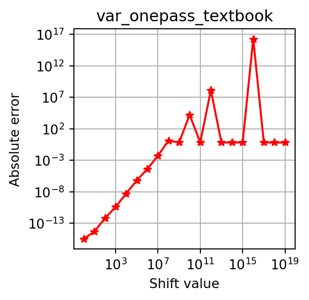

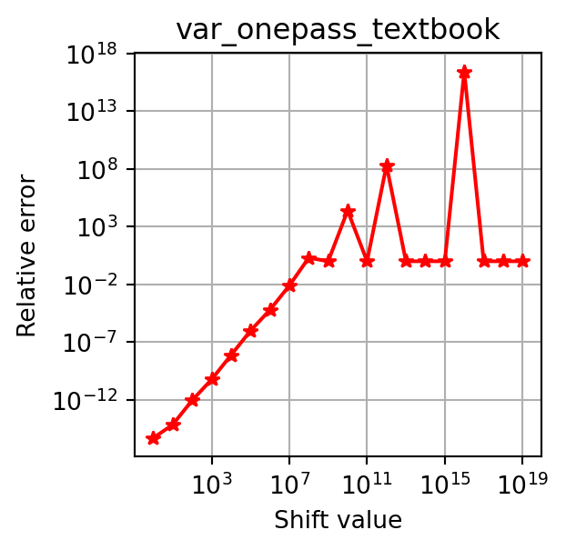
(a) Absolute error

(b) Relative error

Figure 1: Error plots for the one-pass textbook formula.

This instability makes the textbook one-pass formula unsuitable for real-world use.

3 Floating Point Arithmetic

Why does this happen? Because floating-point numbers can only represent a finite number of digits. Squaring a large number, for example, can lose precision:

1000000001.0 ** 2
# 1.000000002000000001e+18

1.000000002e+18

Moreover, floating point numbers cannot exactly represent all values, especially very large numbers, leading to rounding errors.

1000000002000000001.0

1.000000002e+18

Most systems use the IEEE 754 standard. In double precision (64-bit), numbers have 53 bits of precision, so integers larger than 2^{53}-1 (9007199254740991) cannot be represented exactly. For example, adding small increments beyond this threshold reveals precision loss:

print(9007199254740991.0)        # correct
print(9007199254740991.0 + 1.0)  # still correct
print(9007199254740991.0 + 2.0)  # wrong

9007199254740991.0
9007199254740992.0
9007199254740992.0

The hex representation makes this clear:

print(hex(9007199254740991))  # exact
print(hex(9007199254740992))  # exact
print(hex(9007199254740993))  # last bit lost

0x1fffffffffffff
0x20000000000000
0x20000000000001

Large numbers like:

print(hex(1000000002000000001))

0xde0b6b41e999401

also show lost lower bits, which is exactly what causes variance miscalculations.

4 Stable Alternatives

A better one-pass approach is Welford’s algorithm (Welford 1962). Instead of subtracting large similar terms, it incrementally updates the mean \mu_k=\sum_{i=1}^k x_i / k and the squared deviations S_k=\sum_{i=1}^k (x_i - \mu_k)^2 to maintain numerical stability:

\begin{align*} \delta_k &= x_k - \mu_{k-1},\\ \mu_k &= \mu_{k-1} + \delta_k / k,\\ S_k &= S_{k-1} + \delta_k (x_k - \mu_k). \end{align*} \tag{3}

def var_onepass_welford(x):
    n, mu, sd = 0, 0, 0
    for xi in x:
        n += 1
        delta = xi - mu
        mu += delta / n
        sd += delta * (xi - mu)
    return sd / n

Testing again with shifts:

for shift in [1e3, 1e6, 1e9, 1e12]:
    xt = x + shift
    print(f"Shift: {shift:.0e}")
    print(f"One-pass (Welford): {var_onepass_welford(xt)}\n")

Shift: 1e+03
One-pass (Welford): 0.6666666666666666

Shift: 1e+06
One-pass (Welford): 0.6666666666666666

Shift: 1e+09
One-pass (Welford): 0.6666666666666666

Shift: 1e+12
One-pass (Welford): 0.6666666666666666

Welford’s method remains stable even under extreme shifts. Other methods, such as Chan’s algorithm (T. F. Chan, Golub, and LeVeque 1982), are also numerically stable. Classic studies (Ling 1974; Tony F. Chan, Golub, and Leveque 1983) provide detailed comparisons.

References

Chan, T. F., G. H. Golub, and R. J. LeVeque. 1982. “Updating Formulae and a Pairwise Algorithm for Computing Sample Variances.” In COMPSTAT 1982 5th Symposium Held at Toulouse 1982, 30–41. Heidelberg: Physica-Verlag HD. https://doi.org/10.1007/978-3-642-51461-6_3.

Chan, Tony F., Gene H. Golub, and Randall J. Leveque. 1983. “Algorithms for Computing the Sample Variance: Analysis and Recommendations.” The American Statistician 37 (3): 242–47. https://doi.org/10.1080/00031305.1983.10483115.

Ling, Robert F. 1974. “Comparison of Several Algorithms for Computing Sample Means and Variances.” Journal of the American Statistical Association 69 (348): 859–66. https://doi.org/10.1080/01621459.1974.10480219.

Welford, B. P. 1962. “Note on a Method for Calculating Corrected Sums of Squares and Products.” Technometrics 4 (3): 419–20. https://doi.org/10.1080/00401706.1962.10490022.